LM Curve

Table Of Content

LM Curve

Hey Mumbai University SYBA IDOL students! Today, we’re diving into the fascinating world of Macro Economics , exploring about – “LM Curve“. In this class, we are going to talk about an important concept called the LM Curve. Don’t worry if this sounds new — I’ll make sure everything is explained in simple language so everyone can understand.

We will first learn how the LM curve is derived. This means we will look at how the money market works — how income and interest rates are related — and how this relationship helps us draw the LM curve.

After that, we’ll see how both the goods market and the money market can be in balance at the same time. This is shown through something called the IS-LM model, where both the IS curve (from the goods market) and the LM curve (from the money market) come together. This helps us understand how an economy can reach an overall equilibrium.

By the end of today’s session, you will have a clear idea about how these curves work and how they are used to study economic stability.

So, SYBA IDOL Mumbai University students, get ready to unwrap the “LM Curve” with customized IDOL notes just for you. Let’s jump into this exploration together

Question 1 :- How LM curve is derived?

Introduction:
In macroeconomics, the LM Curve is a crucial concept that helps us understand the relationship between the money market and the economy. The acronym “LM” stands for Liquidity Preference and Money Supply. Essentially, the LM Curve represents the various combinations of interest rates and levels of income where the money market is in equilibrium. This equilibrium occurs when the demand for money is equal to the supply of money. Understanding the derivation of the LM Curve is important for grasping how changes in economic factors affect interest rates and income levels within a nation, and how these elements interplay to determine the overall economic equilibrium.

1. Understanding Money Market Equilibrium

The money market is in equilibrium when the demand for real balances (money people want to hold) equals the supply of real balances (money actually available).
The formula for this equilibrium is given by $L = P M$ , where:
$L$ is the demand for real money balances (liquidity preference).
$M$ is the nominal money supply (the total amount of money available).
$P$ is the price level (the average of current prices).
The equation highlights that the supply of real money balances is determined by how much money is available and how much it is worth (adjusted for price level).

2. Demand for Money

The demand for money can be influenced by several factors, prominently including the level of income $Y$ and the interest rate $i$ .
This relationship is captured by the equation: $L = kY - hi$ , where:
$k$ is the responsiveness of money demand to changes in income.
$h$ is the responsiveness of money demand to changes in the interest rate.
Generally, as income increases, people demand more money, but as interest rates rise, the demand for holding money decreases because higher rates incentivize investing in interest-bearing assets.

3. Deriving the LM Curve

To derive the LM Curve, we analyze how different levels of income and interest rates can fulfill the equilibrium condition in the money market.
By rearranging the equation, we can express it in terms of the interest rate: $i = h 1 (kY - P M)$
This equation indicates how the interest rate changes with variations in income while keeping the money supply constant.
By plotting this relationship on a graph with income levels on the X-axis and interest rates on the Y-axis, we get a downward-sloping LM Curve.
The downward slope arises because, at higher income levels, interest rates must be lower to maintain equilibrium. This reflects the inverse relationship between the interest rate and the demand for money.

4. Interpreting the LM Curve

Each point on the LM Curve represents a specific combination of interest rates and income levels that satisfy the money market equilibrium.
As the economy experiences changes (like an increase in income), the demand for money shifts, leading to a new equilibrium at a different point on the curve.
If income increases significantly, the demand for money grows, and without an increase in money supply, interest rates must rise to restore equilibrium. Hence, this shift illustrates the flexibility and responsiveness of the economy to various factors.

5. Shifts in the LM Curve

The LM Curve can shift due to changes in the money supply. For example, if the central bank increases the money supply ( $M$ ), the entire curve shifts to the right, indicating lower interest rates at each income level, promoting economic activity.
Conversely, any decrease in the money supply would shift the LM Curve to the left, resulting in higher interest rates at the same income levels.

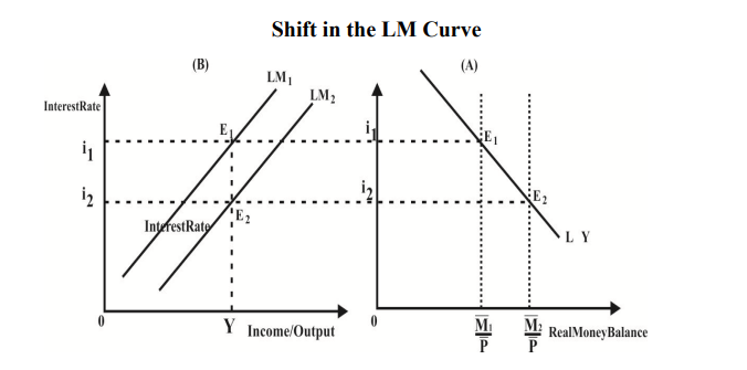
7. Diagram Explanation

Panel A (Right Side): This shows how an increase in real money balances (M/P) from M1P\frac{M_1}{P} to M2P\frac{M_2}{P} leads to a downward movement in the interest rate from i1i_1 to i2i_2, creating a new equilibrium point.
Panel B (Left Side): It shows the LM curve shifting from LM₁ to LM₂. This shift happens because the increase in money supply (seen in Panel A) allows for a higher level of income (Y) at the same interest rate, showing economic expansion.

8. Real-World Example: Imagine the RBI increases the money supply by printing more currency or lowering interest rates. This gives people more cash in hand, making loans cheaper. As a result, consumers spend more, and businesses invest more, which increases income in the economy. The LM curve shifts to the right, showing that the same interest rate can now support a higher level of income.

Conclusion:

The LM Curve is a key concept in macroeconomics. It shows how interest rates and income levels interact in the money market. By learning how it is derived and how it shifts, we get a deeper understanding of how the economy works and how monetary policy can influence growth and stability.

This understanding is especially helpful when we combine the LM Curve with the IS Curve, which represents the goods market, to analyze the overall economic equilibrium using the IS-LM model.

Question 2 :- Show how simultaneous equilibrium is reached in goods market and money market with the help of IS-LM curves.

Introduction:

The interaction between the goods market and the money market is a fundamental concept in macroeconomics. It determines the overall equilibrium level of national income and interest rates in an economy. To analyze this interaction, economists use the IS-LM model, which integrates two key curves:

IS Curve: Represents equilibrium in the goods market
LM Curve: Represents equilibrium in the money market

Understanding how these markets interact to achieve simultaneous equilibrium is crucial to grasp the broader dynamics of economic activity, investment, consumption, and monetary policy. The IS-LM framework helps visualize the relationship between income and interest rates, offering insights into how changes in one market affect the other.

1. Understanding the IS Curve

The IS Curve shows combinations of interest rates and income levels where the goods market is in equilibrium (i.e., Investment = Saving).
It is derived from the equilibrium condition in the goods market:
Y = C + I + G, where
- Y is national income,
- C is consumption,
- I is investment,
- G is government expenditure.
Lower interest rates encourage borrowing and investment, increasing output and income.
Higher interest rates discourage investment, leading to lower income.
Therefore, the IS curve slopes downward, reflecting an inverse relationship between interest rates and income.

2. Understanding the LM Curve

The LM Curve shows combinations of interest rates and income levels that bring equilibrium in the money market.
It is derived from the condition:
Demand for money (L) = Supply of money (M/P)
As income rises, people demand more money for transactions.
To keep money market equilibrium, interest rates must increase.
Thus, the LM curve slopes upward, reflecting a positive relationship between interest rates and income.

3. Simultaneous Equilibrium in IS-LM Framework

The intersection of the IS and LM curves represents the simultaneous equilibrium in both the goods and money markets.
At the equilibrium point (E), we find a unique combination of:
- Interest rate (r₀)
- Income level (Y₀)
  that satisfies both market conditions.
At point E:
- Investment equals saving (IS condition)
- Money demand equals money supply (LM condition)

This is where the economy is in macroeconomic balance — neither the goods market nor the money market has pressure to change.

4. Shifts in Equilibrium and Market Interactions

The IS and LM curves can shift due to changes in fiscal or monetary policy:
- Increase in government spending → IS curve shifts right → Higher income and interest rates
- Increase in money supply by central bank → LM curve shifts right → Lower interest rates and higher income
These shifts show how the goods and money markets are interlinked.
A change in one market leads to adjustments in the other.
Policymakers use these dynamics to guide the economy toward desired levels of employment, output, and price stability.

5. Real-World Implications of IS-LM Equilibrium

The IS-LM model helps explain how:
- An increase in consumer confidence shifts the IS curve right
- A reduction in interest rates by the RBI lowers the LM curve
It also allows economists to predict outcomes of:
- Tax reforms,
- Interest rate changes, and
- Government spending programs

Understanding the IS-LM equilibrium enables students and economists to analyze the impact of combined fiscal and monetary policies on real economic outcomes.

6. Diagram:-

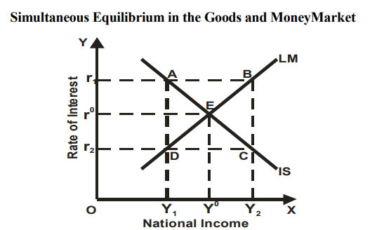
7. Diagram Explanation
- Point E is the equilibrium where both the goods market (IS) and money market (LM) are in balance.
- At point A: Interest rate is high (r₁), leading to excess supply in the goods market
- At point C: Interest rate is low (r₂), leading to excess demand in the money market
- Only at point E (where IS and LM intersect) is there simultaneous equilibrium with no market pressure for change

Conclusion:-

The IS-LM model serves as a vital tool to understand how macroeconomic equilibrium is achieved. It shows the interconnectedness of the real and monetary sectors and provides insights into how policymakers can use fiscal and monetary tools to stabilize the economy.

Important Note for Students :– Hey everyone! All the questions in this chapter are super important!